Here I present a simple example for High-harmonic generation on a 1-dimensional periodic chain with the octopus code.
Hereafter the ground-state input, I used the DOJO pseudo-potential with PBE functional:
CalculationMode = gs
UnitsOutput = ev_angstrom
ExperimentalFeatures = yes
PeriodicDimensions = 1
Spacing = 0.5
%LatticeParameters
2.0*angstrom | 4*angstrom | 4*angstrom
%
%Species
"H" | species_pseudo | file | "H.dojo.upf"
%
%Coordinates
"H" | -0.3707*angstrom | 0.0 | 0.0
"H" | 0.3707*angstrom | 0.0 | 0.0
%
%KPointsGrid
24 | 1 | 1
%
KPointsUseSymmetries = yes
%SymmetryBreakDir
1 | 0 | 0
%
then the real-time input with the laser field:
CalculationMode = td
FromScratch = yes
FromScratch = yes
UnitsOutput = ev_angstrom
ExperimentalFeatures = yes
PeriodicDimensions = 1
Spacing = 0.5
%LatticeParameters
2.0*angstrom | 4*angstrom | 4*angstrom
%
# TheoryLevel = independent_particles
%Species
"H" | species_pseudo | file | "H.dojo.upf"
%
%Coordinates
"H" | -0.3707*angstrom | 0.0 | 0.0
"H" | 0.3707*angstrom | 0.0 | 0.0
%

# Frequency corresponding to 0.75 eV.
omega = 0.02756196963750000000
period = 2*pi/omega
stime = 10*period

TDPropagationTime = stime+period
TDPropagator = exp_mid
TDExponentialMethod = lanczos
TDExpOrder = 10
TDTimeStep = 0.1
%TDExternalFields
vector_potential | 1 | 0 | 0 | omega | "envelope_function"
%
electric_amplitude = -c/omega*(sqrt(1*10^9)/sqrt(3.509470*10^16)) # in atomic units
%TDFunctions
"envelope_function" | tdf_from_expr | "electric_amplitude*(sin(pi/stime*t))^2*(1-step(t-stime))"
%
%TDOutput
laser
total_current
%
%KPointsGrid
24 | 1 | 1
%
%SymmetryBreakDir
1 | 0 | 0
%
KPointsUseSymmetries = yes
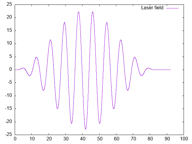
you can plot the laser field with the gnuplot and the command:
p 'td.general/laser' u 1:3 w l
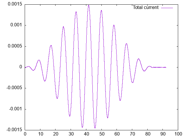
and the total current with:
p 'td.general/total_current' u 1:3 w l
then the current can be post-process with the command oct-harmonic-spectrum with the input:
omega = 0.02756196963750000000
PropagationSpectrumMaxEnergy = 30*omega
PropagationSpectrumEnergyStep = omega/20
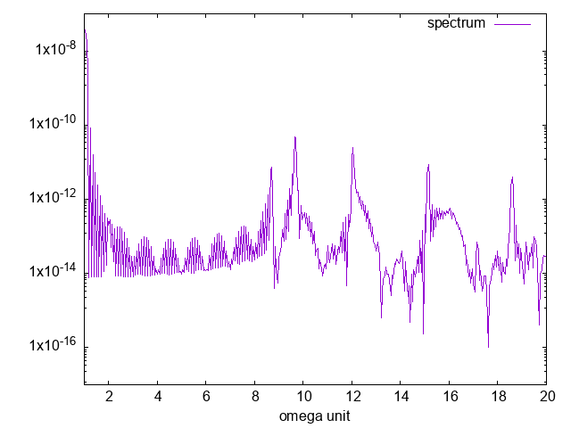
the spectrum is written in the file hs-mult.x, and you can plot it in logarithmic scale:


