Linear response in real-time
First of all compile QuantumEspresso and Yambo/Lumen. If you have problems in compilation please have a look to: compiling yambo.
The tutorial on linear response from real-time Schödinger equation is divided in 8 steps:
1) DFT calculations
In Lumen (and Yambo) all quantities are written in a basis of the Kohn-Sham(KS) eigenvalues and eigenvectors. In order to generate this basis we use a DFT code in plane wave as Abinit or QuantumEspresso(QE).
In this example we will consider a single later of hexagonal boron nitrite (hBN), the input files available here (QE_inputs or ABINIT_inputs). The first input file is a self-consistent(SCF) calculation that is used to generate the density of the system. The second input file is a non-self consistent(NSCF) calculation to diagonalize the KS Hamiltonian, that depends from the density of the first run, on for a given number of bands and k-points. Notice that parameters in the NSCF calculation determine the number of k-points and the maximum number of bands that can be used in Lumen. Run these calculation with the command:
for QuantumEspresso:
for Abinit:
Notice that in the NSCF file of QuantumEspresso we use the flag force_symmorphic=.true. to exclude the non-symmorphic symmetries that are not supported by Lumen(Yambo), in Abinit the same option is activated by the flag symmorphi 0.
2) Import the wave-functions
If you used QuantumEspresso go in the folder bn.save, in the ABINIT case all file are already in the main folder. Then import the wave-function with the command
for QuantumEspresso:
for Abinit:
4) Setup
Generate the setup input file with the command yambo_nl -i -V RL -F setup.in, then run yambo_nl -F setup.in. You can reduce the number of G-vectors in the setup in such a way to speed up calculations. I advise to reduce G-vector to 1000 (about 50% the initial ones).
5) Reduce symmetries
Since in real-time simulation we introduce a finite electric field in the Hamiltonian, the number of the symmetries of the original system is reduced due to the presence of this field. Using the tool ypp -y to generate the input file:
Set the external field in the y direction and uncomment the Time Reversal flag, as shown in red above. Run ypp and it will create a new folder called FixSymm with the reduced symmetries wave-functions.
6) Setup again
Go in the FixSymm directory and run the setup again yambo_nl -F ../setup.in. Now everything is ready for the real-time simulations!
7) Real-time dynamics
In order to calculate linear-response in real-time we will perturb the system with a delta function in time external field. Use the command yambo_nl -u -F input_lr.in to generate the input:
We set the verbosity to "high" in such a way to print real-time output files.
We set the differential equation integrator to INVINT that is faster bul less accurate than the default(see PRB 88, 235113). This integrator is ok in case of independent partcicles but I advise you to use CRANKNIC integrator when correlation effects are present. Now run yambo_nl -F input_lr.in
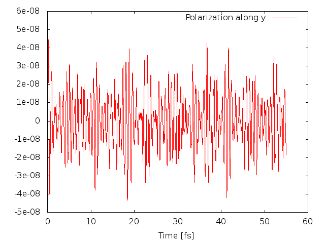
The code will produce different files: o.polarization_F1 that contains the polarization, o.external_potential_F1 the external field we used, and finally r_optics_nloptics a report with all information about the simulation. If you plot the third column of o.polarization_F1 versus the first one (time variable) you will get the time-dependent polarization along the y direction:

8) Analyze the results
Now we can use ypp_nl -u to analyze the results:
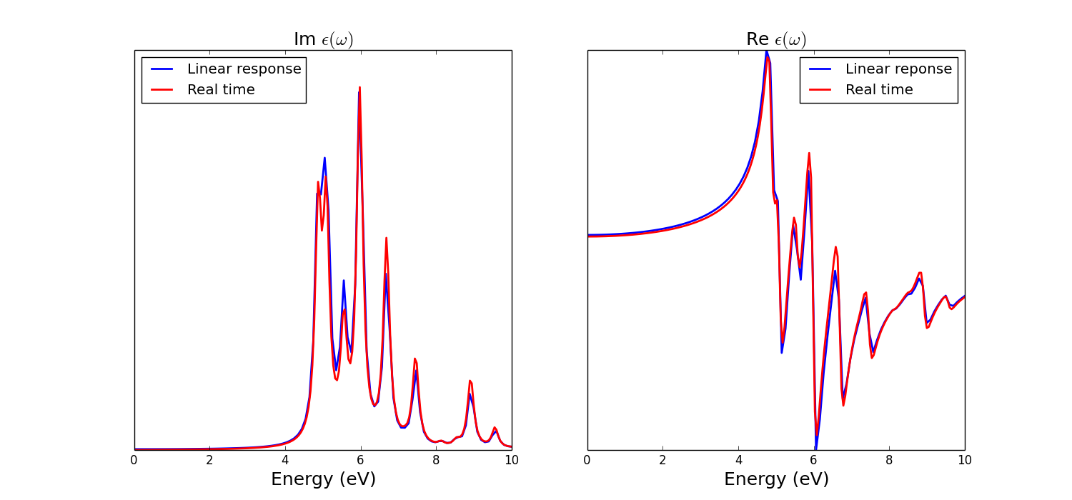
Now we can plot the dielectric constant and compare it with linear response:

The input for the linear response can be downloaded here. Notice that in a real-time simulation we obtain directly the \( \chi(\omega) = \frac{P(\omega)}{E(\omega)} \) that is realted to the dielectric constant from the relation $$\epsilon(\omega) = 1 + 4 \pi \chi(\omega) $$
The tutorial on linear response from real-time Schödinger equation is divided in 8 steps:
1) DFT calculations
In Lumen (and Yambo) all quantities are written in a basis of the Kohn-Sham(KS) eigenvalues and eigenvectors. In order to generate this basis we use a DFT code in plane wave as Abinit or QuantumEspresso(QE).
In this example we will consider a single later of hexagonal boron nitrite (hBN), the input files available here (QE_inputs or ABINIT_inputs). The first input file is a self-consistent(SCF) calculation that is used to generate the density of the system. The second input file is a non-self consistent(NSCF) calculation to diagonalize the KS Hamiltonian, that depends from the density of the first run, on for a given number of bands and k-points. Notice that parameters in the NSCF calculation determine the number of k-points and the maximum number of bands that can be used in Lumen. Run these calculation with the command:
for QuantumEspresso:
pw.x -inp BNsheet.scf.in  > output_scf
pw.x -inp BNsheet.nscf.in > output_nscf
for Abinit:
abinit < hBN.files > output_hBN
Notice that in the NSCF file of QuantumEspresso we use the flag force_symmorphic=.true. to exclude the non-symmorphic symmetries that are not supported by Lumen(Yambo), in Abinit the same option is activated by the flag symmorphi 0.
2) Import the wave-functions
If you used QuantumEspresso go in the folder bn.save, in the ABINIT case all file are already in the main folder. Then import the wave-function with the command
for QuantumEspresso:
p2y
for Abinit:
a2y -F hbn_out_DS2_KSS
4) Setup
Generate the setup input file with the command yambo_nl -i -V RL -F setup.in, then run yambo_nl -F setup.in. You can reduce the number of G-vectors in the setup in such a way to speed up calculations. I advise to reduce G-vector to 1000 (about 50% the initial ones).
5) Reduce symmetries
Since in real-time simulation we introduce a finite electric field in the Hamiltonian, the number of the symmetries of the original system is reduced due to the presence of this field. Using the tool ypp -y to generate the input file:
fixsyms                      # [R] Reduce Symmetries
% Efield1
 0.00     | 1.00     | 0.00     |        # First external Electric Field
%
% Efield2
 0.00     | 0.00     | 0.00     |        # Additional external Electric Field
%
#RmAllSymm                   # Remove all symmetries
RmTimeRev                   # Remove Time Reversal
Set the external field in the y direction and uncomment the Time Reversal flag, as shown in red above. Run ypp and it will create a new folder called FixSymm with the reduced symmetries wave-functions.
6) Setup again
Go in the FixSymm directory and run the setup again yambo_nl -F ../setup.in. Now everything is ready for the real-time simulations!
7) Real-time dynamics
In order to calculate linear-response in real-time we will perturb the system with a delta function in time external field. Use the command yambo_nl -u -F input_lr.in to generate the input:
nlinear                      # [R NL] Non-linear optics
NL_Threads= 1                # [OPENMP/NL] Number of threads for nl-optics
% NLBands
  3 |  6 |                   # [NL] Bands
%
NLstep=   0.0100       fs    # [NL] Real Time step length
NLtime=55.000000      fs    # [NL] Simulation Time
NLverbosity= "high"           # [NL] Verbosity level (low | high)
NLintegrator= "INVINT"       # [NL] Integrator ("EULEREXP/RK4/RK2EXP/HEUN/INVINT/CRANKNIC")
NLCorrelation= "IPA"         # [NL] Correlation ("IPA/HARTREE/TDDFT/LRC/JGM/SEX/HF")
NLLrcAlpha= 0.000000         # [NL] Long Range Correction
% NLEnRange
 0.200000 | 8.000000 | eV    # [NL] Energy range
%
NLEnSteps= 1                 # [NL] Energy steps
NLDamping= 0.000000    eV    # [NL] Damping
% ExtF_Dir
 0.000000 | 1.000000 | 0.000000 |        # [NL ExtF] Versor
%
ExtF_kind= "DELTA"         # [NL ExtF] Kind(SIN|SOFTSIN|RES|ANTIRES|GAUSS|DELTA|QSSIN)
The standard input of Lumen is thought for non-linear response so we have to
change some parameters in order to calculate the linear response.
Set the field direction along y, the field type to DELTA, the length of the simulation to 55 fs, number of bands from 3 to 6 dephasing to zero and the number of energy steps to one, as shown above in red.We set the verbosity to "high" in such a way to print real-time output files.
We set the differential equation integrator to INVINT that is faster bul less accurate than the default(see PRB 88, 235113). This integrator is ok in case of independent partcicles but I advise you to use CRANKNIC integrator when correlation effects are present. Now run yambo_nl -F input_lr.in
The code will produce different files: o.polarization_F1 that contains the polarization, o.external_potential_F1 the external field we used, and finally r_optics_nloptics a report with all information about the simulation. If you plot the third column of o.polarization_F1 versus the first one (time variable) you will get the time-dependent polarization along the y direction:

8) Analyze the results
Now we can use ypp_nl -u to analyze the results:
nonlinear                    # [R] NonLinear Optics Post-Processing
Xorder= 1                    # Max order of the response functions
% TimeRange
-1.000000 |-1.000000 | fs    # Time-window where processing is done
%
ETStpsRt= 200                # Total Energy steps
% EnRngeRt
  0.00000 | 10.00000 | eV    # Energy range
%
DampMode= "LORENTZIAN"             # Damping type ( NONE | LORENTZIAN | GAUSSIAN )
DampFactor=  0.10000   eV    # Damping parameter
where we set a lorentzian smearing corresponding to 0.1 eV. Notice that due to the finite time of our simulation a smearing is always necessary to Fourier transform the result. Then we run ypp_nl and obtain the following files: the dielectric constant along the field direction o.YPP-eps_along_E, the EELS along the same direction o.YPP-eels_along_E, and the damped polarization o.YPP-damped_polarization.
Now we can plot the dielectric constant and compare it with linear response:

The input for the linear response can be downloaded here. Notice that in a real-time simulation we obtain directly the \( \chi(\omega) = \frac{P(\omega)}{E(\omega)} \) that is realted to the dielectric constant from the relation $$\epsilon(\omega) = 1 + 4 \pi \chi(\omega) $$